Football goals and coin flips: discovering the law of rare events
Ever felt excited for discovering something that is already kinda known? Not necessarily for the discovery itself, but because you achieved it on your own and actually overcame an obstacle with it.
This is how I feel about this story, and hopefully you will too. Starting from a small puzzle about football, we’re going to build the solution from scratch and see how -without knowing it- we just applied the law of rare events.
The problem
In the English Premier League, 2.66 goals are scored per football match on average. What’s the probability of a match with more than 6 goals?
Intuitively, it feels like we should be able to answer, even with this single piece of given information. But it’s not that straightforward. The figure below shows three potential solutions to our problem, all consistent with the given mean goals per match (2.66).
Figure 1: Three potential solutions to the problem. Points: probabilities of a match with specified number of goals; green points: probabilities of a match with more than 6 goals; P(more than 6 goals): sum of probabilities for more than 6 goals in each scenario, i.e. solutions to our problem; dashed line: mean goals per match.
And these are just 3 scenarios - who knows if the correct solution is one of them or another one entirely?
Let’s get started.
Strategy
We are equipped with the mean goals per match and almost no Statistics background. We just know what a mean and what a probability is. We compensate that with a critical mind and some data analysis skills.
A good start is to define our only piece of given information - the mean goals per match:
mean.goals <- 2.66
Code explanation
- The
<-operator assigns the value 2.66 to the variablemean.goals. From now on, we’ll refer to this value by this name for calculations.
In this blog’s very first post, I argued that questions about probability of outcomes can be flipped to questions about tangible data. So let’s rephrase the question:
What’s the frequency (percentage) of matches with more than 6 goals?
The idea is to analyze the goals of simulated football matches. This should give us an approximation of the true probability.
Each simulated match should have a random but realistic number of goals, somehow based on our given mean. In other words, the randomness must still follow a pattern.
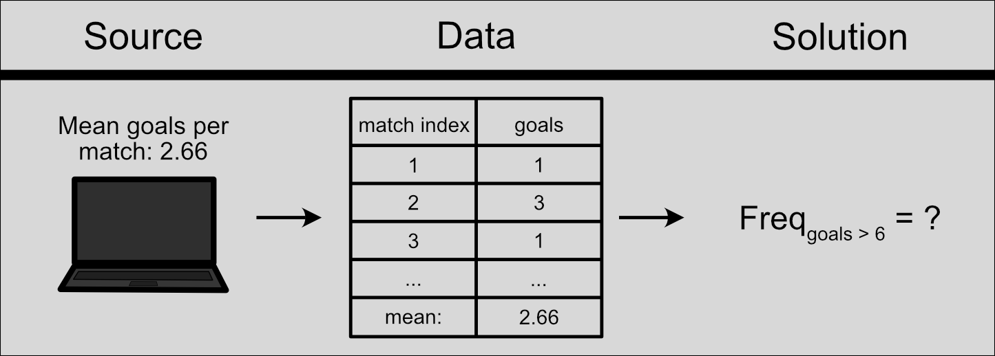
Figure 2: Data-driven approach to find the solution using simulated football matches.
The question is, can we actually create this data?
Football goal simulation: how to create patterned randomness
Let’s define what a goal is to us: an event that may occur a number of times -including 0 times- within a match. In reality, a goal can occur at any moment in the continuous duration of a match (90 minutes).
But there’s a problem: I don’t know how to simulate random events in truly continuous time. So we’ll go for the next best option: divide each match into a grid of short, indivisible time chunks. Each of them can have either 0 or 1 goal scored - never 2 or more goals.
If we have n time chunks in each match:
-
The maximum number of goals we can have is n
-
Each time chunk has equal duration (in minutes):
\(\frac{match~time}{n} = \frac{90}{n}\) -
Each time chunk has equal probability of a scored goal. Perhaps it makes sense that this probability is:
\(p_{goal} = \frac{mean~goals}{n} = \frac{2.66}{n}\) -
Following that, the probability of no-goal in each time chunk is:
\(p_{no~goal} = 1 - p_{goal} = 1 - \frac{2.66}{n}\)
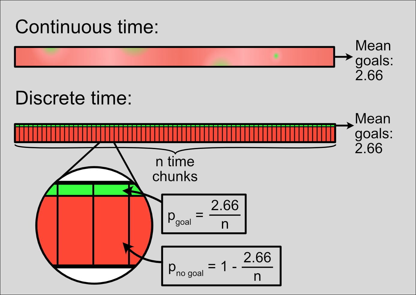
Figure 3: Dividing a continuous match duration into discrete time chunks with equal probability of a scored goal.
It’s time for our first decision: how many time chunks should we divide a match into?
We should definitely have more than 2. Otherwise we’d limit ourselves to strictly 2 goals or less. Besides, the probability \(p_{goal} = \frac{2.66}{2}\) would be higher than 1 and wouldn’t even make sense as a probability.
The more time chunks, the better they should resemble continuous time, so let’s be generous. I decide to set each time chunk to 1 minute. This means 90 time chunks per match.
Let’s begin. The code below creates a table named simulated.match.data, representing 100,000 matches divided in 90 time chunks. Each row will represent a time chunk.
# Load data.table library
library(data.table)

# Create a table representing all time chunks of 100,000 matches
simulated.match.data <- CJ(match.index=seq_len(100000),
                           time=seq_len(90))

simulated.match.data
## Key: <match.index, time>
##          match.index  time
##                <int> <int>
##       1:           1     1
##       2:           1     2
##       3:           1     3
##       4:           1     4
##       5:           1     5
##      ---
## 8999996:      100000    86
## 8999997:      100000    87
## 8999998:      100000    88
## 8999999:      100000    89
## 9000000:      100000    90
Code explanation
-
We want to reproduce all 90 time chunks (indexed from 1 to 90) of 100,000 matches (indexed from 1 to 100,000). This is easy to create with the
CJfunction of thedata.tablepackage. -
First, we create these two sequences (1 to 100,000 and 1 to 90) with the
seq_lenfunction (see relevant section in Sequences). -
These two sequences are given as input to
CJ, which creates a cross-join table with 100,000 times 90 (= 9 million) rows.
In this case, the probability for a scored goal in each time chunk is:
\(p_{goal} = \frac{mean~goals}{n} = \frac{2.66}{90} \approx 0.0296\)
Similarly, the probability of no-goal in each time chunk is: \(p_{no~goal} = 1 - p_{goal} \approx 1 - 0.0296 = 0.9704\)
Let’s recreate this randomness to our simulated matches. The code below applies these probabilities to each time chunk and creates a new field named scored.goal, which signifies whether or not a goal has been scored.
# Initialize random seed
set.seed(seed=1)

# Assign goal or no-goal to each time chunk of each match
simulated.match.data[
  ,scored.goal:=sample(x=c(TRUE,FALSE),
                       size=.N,
                       replace=TRUE,
                       prob=c(mean.goals/.N,
                              1-mean.goals/.N)),
  by=match.index]

simulated.match.data
## Key: <match.index, time>
##          match.index  time scored.goal
##                <int> <int>      <lgcl>
##       1:           1     1       FALSE
##       2:           1     2       FALSE
##       3:           1     3       FALSE
##       4:           1     4       FALSE
##       5:           1     5       FALSE
##      ---
## 8999996:      100000    86       FALSE
## 8999997:      100000    87       FALSE
## 8999998:      100000    88       FALSE
## 8999999:      100000    89       FALSE
## 9000000:      100000    90       FALSE
Code explanation
-
The
set.seedfunction initializes the conditions for random processes, ensuring reproducible results. See details on initializing seed. -
We want to affect all rows of our table, so we don’t apply any row filter. Thus the 1st argument in square brackets -used for row filtering- remains blank (hence the comma
,immediately after the opening bracket[). -
We create the
scored.goalfield using the:=operator, specific to thedata.tablepackage (see relevant section in Column operations). -
The
samplefunction randomly draws from the two elements in a “bucket”:TRUEfor goal orFALSEfor no-goal. Parameters (arguments) set for this particular case:-
x: The “bucket” itself. A vector with the valuesTRUEandFALSE, combined together with thec()function. -
size: The number of draws. In this case.N, i.e. the number of time chunks per match (see below). -
.Nis a special symbol in thedata.tablesyntax, counting the number of rows (time chunks). Here,.Ncounts the time chunks of each individual match (not the whole table), because of the grouping argumentby=match.index. -
replace=TRUE: Sets random drawing with replacement. This means that after a random option is drawn fromx, it is replaced in the “bucket”, so the probabilities of each option remain the same (see relevant section in Random samples). -
prob: The probabilities forTRUEorFALSE. They are calculated on the spot (mean.goals/.Nand1-mean.goals/.N) and combined in a vector.
-
We now have data for 100,000 simulated matches! Of course most of our 9 million simulated time chunks don’t have a scored goal (FALSE). Rest assured though, we’ll get to the scored goals right away.
Pre-processing of simulated data
Our simulated data is not yet arranged to show what we want. We don’t really care about when exactly each goal was scored, but how many goals were scored in each match.
The code below counts all the goals for each simulated match and stores the results in a new table named simulated matches.
simulated.matches <- simulated.match.data[
  ,.(goals=sum(scored.goal)),
  by=match.index]

simulated.matches
## Key: <match.index>
##         match.index goals
##               <int> <int>
##      1:           1     1
##      2:           2     4
##      3:           3     0
##      4:           4     6
##      5:           5     2
##     ---
##  99996:       99996     2
##  99997:       99997     2
##  99998:       99998     0
##  99999:       99999     0
## 100000:      100000     2
Code explanation
-
We create and display an aggregate table, with a field
goals, which sums the goals for each simulated match. -
For the total goals we need to count the
TRUEvalues inscored.goal. So we simplysumthe fieldscored.goal.TRUEis handled as 1 andFALSEas 0, see Handling logical values as numbers. -
We group the rows (time chunks) of each individual match by setting the grouping argument
bytomatch.index.
Now that have our simulated data exactly as we want it, let’s proceed to analyze it.
Data analysis
First, a reality check: does our data agree with our one and only assumption - that mean goals per match = 2.66?
# Mean goals per match in simulated matches
simulated.matches[,mean(goals)]
## [1] 2.66098
Code explanation
We simply calculate and display the mean of goals for all matches. As we want to include all matches, the first argument within square brackets is left blank ([,...]).
So our simulation seems to have worked well. If the mean we got here was very off, it would mean we screwed up at some point.
We’ll next count the matches for each number of goals - how many matches with 0 goals, how many with 1 goal, and so on. This will be in both absolute amount and frequency (percentage).
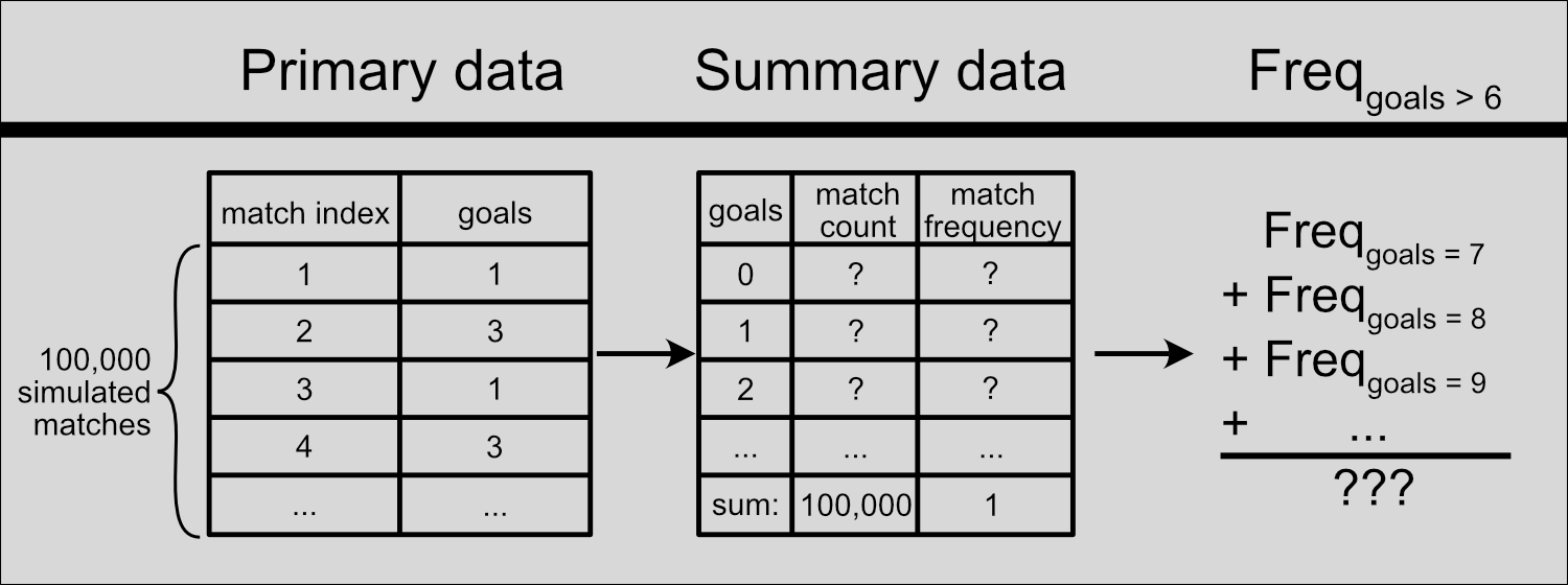
Figure 4: Data analysis procedure.
# Count the matches for each number of goals
simulated.summary <- simulated.matches[
  ,.(match.count=.N),
  by=goals]

# Calculate corresponding frequencies
simulated.summary[,match.frequency:=match.count/sum(match.count)]

# Sort rows in ascending order for goals
simulated.summary |> setorder(goals)

# Show the resulting table
simulated.summary
##     goals match.count match.frequency
##     <int>       <int>           <num>
##  1:     0        6751         0.06751
##  2:     1       18365         0.18365
##  3:     2       24954         0.24954
##  4:     3       22285         0.22285
##  5:     4       14786         0.14786
##  6:     5        7760         0.07760
##  7:     6        3331         0.03331
##  8:     7        1276         0.01276
##  9:     8         364         0.00364
## 10:     9          92         0.00092
## 11:    10          30         0.00030
## 12:    11           4         0.00004
## 13:    12           2         0.00002
Code explanation
We create a new aggregate table for the summarized data (simulated.summary) to calculate the frequency of matches with each number of goals (0, 1, 2, and so on.)
-
The
match.countfield counts the rows (.N) of each match category. Matches of the same number of goals are grouped together by setting the grouping factorbytogoals. -
To calculate the frequency of each match category (
match.frequency), we divide the absolute count (match.count) by the number of total matches (sum(match.count)). -
As a finishing touch, we use the
setorderfunction of thedata.tablepackage to sort the rows of the summary table by ascending total goals.
Now we can finally answer the question:
What’s the frequency of matches with more than 6 goals?
Let’s see how the resulting frequencies look like. The green bars in the following plot correspond to the matches we’re interested in:
Figure 5: Frequencies of simulated matches with different number of goals. Green: frequencies of matches with more than 6 goals; dashed line: given mean goals per match (2.66). Interactive plot: hover mouse over bars to see values.
The frequency of matches with more than 6 goals is simply the sum of all green bars. we can easily calculate that from our summary data:
# Simulated matches
simulated.summary[goals>6,sum(match.frequency)]
## [1] 0.01768
Code explanation
We want to add together the frequencies of all matches with more than 6 goals. So we apply this row filter (goals>6) and sum together the match.frequency field for these rows.
The frequency of simulated matches with more than 6 goals is quite low, around 0.0177 or 1.77%.
Seems reasonable as an approximation of the truth. What is the true probability we’re looking for though?
It’s time to lift the curtain and put all the work we just did in some much-needed Statistics context.
Context: the statistics of random events
By simulating football matches, we tried to see the behavior of a random value: the number of scored goals. Specifically, we caught a glimpse of how it is distributed.
Scored goals per match is just one example of this pattern. It models any kind of random events in a specified time: goals per match, cars crossing a bridge per hour, phone calls per day, volcanic eruptions per year, and beyond. And it has a name: the Poisson distribution.
Discrete events in continuous time: the Poisson distribution
The Poisson distribution tells us “how probable it is for an event to happen X times in a fixed interval” and it’s is defined by only 1 parameter: the mean number of events within the interval.
The mean is symbolized as the Greek letter λ (lambda) and the distribution itself is symbolized as \(Pois(λ)\).
That’s why we only needed to know the mean goals per match. So the Poisson distribution for goals per match is symbolized as \(Pois(λ=2.66)\). In the plot below we can see how the Poisson probabilities look like, compared to our simulated match frequencies:
Figure 6: Poisson probability distribution for λ = 2.66 (points) and simulated match frequencies (bars) for number of scored goals. Green bars: frequencies of matches with more than 6 goals; dashed line: mean goals per match (2.66). Interactive plot: hover mouse over bars to see values.
Answering the problem
Armed with this, let’s give a final answer to the original question: what’s the Poisson probability of a match with more than 6 goals.
To calculate it, we need to sum together all probabilities of \(Pois(λ=2.66)\) for X > 6. The answer to this comes from Statistics and specifically the cumulative distribution function:
# Poisson probability for X > 6
ppois(q=6,lambda=mean.goals,lower.tail=FALSE)
## [1] 0.01915806
Code explanation
ppois is a built-in function of R that calculates the summed Poisson probability (cumulative probability) over or under a specified point. In this case:
-
lambda=2.66specifies the mean of the distribution. -
q=6specifies the point to be 6. -
lower.tail=FALSEspecifies that we want the sum of all probabilities over that point.
So our approximation based on simulated matches (Freqgoals>6 = 0.0177) was somewhat off from the Poisson probability. And for good reason: if you recall, we could not simulate continuous time.
Instead, we decided to divide each match into a grid of short time chunks, where a goal may or may not be scored.
In other words, we treated a football match as a series of success/failure trials. This actually generates something else: the binomial distribution.
From continuous to discrete time: the binomial distribution
The binomial distribution tells us “how probable it is to have X successful trials in n total trials”. It’s symbolized as \(B(n,p)\) and defined by 2 parameters: the number of trials (n) and the probability of success in each trial (p).
Take the simplest example: a series of random coin flips, where we assign heads as “success” and tails as “failure”. The number of successes (X) follows the binomial distribution \(B(n,p=0.5)\).
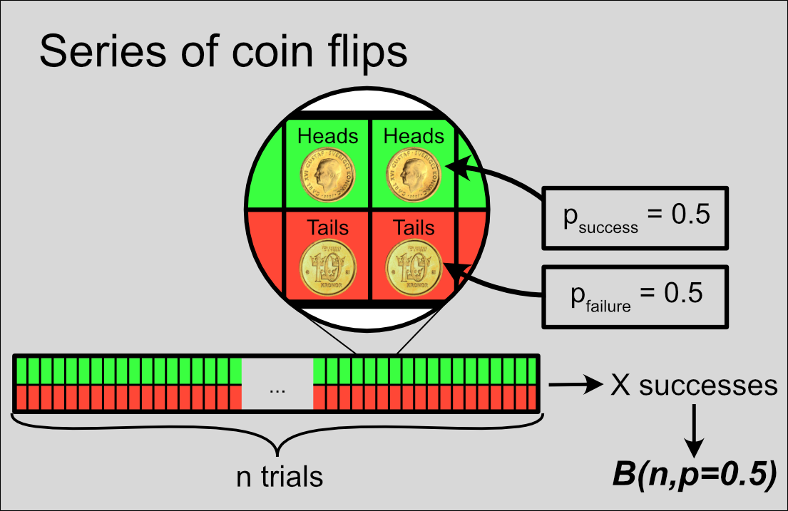
Figure 7: A series of n coin flips. Green and red: probabilities of success (heads) and failure (tails) for each trial.
Try adjusting the number of trials in the figure below, and see how it affects the distribution and the mean number of successes.
Figure 8: Binomial probability distribution for the number of successes (heads) in a series of n coin flips. Dashed line: mean number of successes; green bar: probability of success (heads) in each trial. Adjust the number of total coin flips with the bottom slider.
Football matches as series of goal/no-goal trials
Treating a football match as a series of goal/no-goal trials leads to a binomial distribution, but with a twist: as we increase the number of time chunks (n), the mean number of goals (λ) has to remain fixed. So the probability of goal in each time chunk (p) has to decrease.
| Increasing n | Coin flips | Match time chunks |
|---|---|---|
| psuccess in each trial: | Fixed | $\frac{λ}{n}$ (decreased) |
| Mean number of successes: | psuccess \(\cdot\) n (increased) |
Fixed |
This is essentially what we tried to find with our simulated matches:
pbinom(q=6,size=90,prob=mean.goals/90,lower.tail=FALSE)
## [1] 0.01746448
Code explanation
pbinom is just like ppois, but for the binomial distribution: a built-in function that calculates the cumulative probability over or under a specified point. In this case:
-
q=6specifies the point to be 6. -
size=90specifies the number of trials. -
prob=mean.goals/90specifies the probability of success in each trial. -
lower.tail=FALSEspecifies that we want the sum of all probabilities over that point.
This is much closer to our initial result (0.0177), because this is exactly what we were trying to simulate. The small deviation is simply because of the number of matches we simulated (100,000). We’d be even closer with more simulated matches.
This peculiar binomial distribution approaches a very particular shape. Try adjusting the number of time chunks in the figure below, and see what happens:
Figure 9: Probability distributions for the number of goals in a football match. Grey bars: binomial distribution; black points: Poisson distribution; dashed vertical line: mean goals per match (2.66); green bar: probability of a goal in each time chunk. Adjust the number of time chunks with the bottom slider.
If the mean number of successes is fixed, the binomial distribution approaches the Poisson distribution. A bit more formally: as \(n \to \infty\), \(B(n,p = \frac{λ}{n}) \to Pois(λ = n \cdot p)\)
This link between the binomial and the Poisson distribution is the Poisson limit theorem. Because p gets gradually lower (success becomes more rare), it’s also known as the law of rare events.
The point of learning by discovery
I did not start out looking to discuss the Poisson limit theorem. I just wanted to recreate the Poisson distribution with computer simulations. But I couldn’t simulate random events in continuous time, so I re-discovered it by trying to solve this problem.
This is an inductive approach: going from a specific case \(\to\) a general principle.
Circling back to the initial quote, the exact opposite -deduction- is quite common as a teaching approach: describing general principles \(\to\) solving specific problems. This may allow more rigorous and complete coverage of possible cases, but it has been questioned as a teaching approach.1
Inductive teaching creates a need to find and learn the general principle. It also helps the student associate learning with the joy of discovery - and maybe have fun while they’re at it.2
And that’s what this post and this whole blog are about.
Session info
## R version 4.6.0 (2026-04-24 ucrt)
## Platform: x86_64-w64-mingw32/x64
## Running under: Windows 11 x64 (build 26200)
##
## Matrix products: default
##   LAPACK version 3.12.1
##
## locale:
## [1] LC_COLLATE=English_United States.utf8
## [2] LC_CTYPE=English_United States.utf8
## [3] LC_MONETARY=English_United States.utf8
## [4] LC_NUMERIC=C
## [5] LC_TIME=English_United States.utf8
##
## time zone: Europe/Stockholm
## tzcode source: internal
##
## attached base packages:
## [1] stats     graphics  grDevices utils     datasets  methods   base
##
## other attached packages:
## [1] transformr_0.1.5    gganimate_1.0.11    extraDistr_1.10.0.3
## [4] plotly_4.12.0       ggthemes_5.2.0      ggplot2_4.0.3
## [7] data.table_1.18.2.1 blogdown_1.23
##
## loaded via a namespace (and not attached):
##  [1] sass_0.4.10        generics_0.1.4     tidyr_1.3.2        class_7.3-23
##  [5] KernSmooth_2.23-26 lpSolve_5.6.23     stringi_1.8.7      hms_1.1.4
##  [9] digest_0.6.39      magrittr_2.0.5     evaluate_1.0.5     grid_4.6.0
## [13] RColorBrewer_1.1-3 bookdown_0.46      fastmap_1.2.0      jsonlite_2.0.0
## [17] progress_1.2.3     e1071_1.7-17       DBI_1.3.0          httr_1.4.8
## [21] purrr_1.2.2        crosstalk_1.2.2    viridisLite_0.4.3  scales_1.4.0
## [25] tweenr_2.0.3       lazyeval_0.2.3     jquerylib_0.1.4    cli_3.6.6
## [29] rlang_1.2.0        crayon_1.5.3       units_1.0-1        withr_3.0.2
## [33] cachem_1.1.0       yaml_2.3.12        otel_0.2.0         tools_4.6.0
## [37] dplyr_1.2.1        vctrs_0.7.3        R6_2.6.1           proxy_0.4-29
## [41] classInt_0.4-11    lifecycle_1.0.5    stringr_1.6.0      htmlwidgets_1.6.4
## [45] pkgconfig_2.0.3    pillar_1.11.1      bslib_0.10.0       gtable_0.3.6
## [49] glue_1.8.1         Rcpp_1.1.1-1.1     sf_1.1-0           xfun_0.57
## [53] tibble_3.3.1       tidyselect_1.2.1   rstudioapi_0.18.0  knitr_1.51
## [57] farver_2.1.2       htmltools_0.5.9    rmarkdown_2.31     compiler_4.6.0
## [61] prettyunits_1.2.0  S7_0.2.2           gifski_1.32.0-2