The birthday problem — Part 3: Calculating in steps

“Good, fast, cheap. Choose two.” In other words, quality is often expensive and takes time. And sometimes quick and cheap solutions of lower quality are sufficient.

This choice is the point of this series on the birthday problem:

What’s the probability that two students in a classroom share a common birthday?

After failing in part 1 due to an unreasonably expensive method, we took a cheaper shortcut in part 2 and got approximate results as a trade-off.

In this final part, we’ll spend some time understanding the problem to calculate precise results.

Previously in the series #

So far, we’ve bypassed the problem’s nature and reshaped it into one of data engineering:

• Part 1: Counting. We tried to recreate and analyze all possible combinations of birthdays. This gives precise results but needs huge amounts of computer memory. So we could only find results for 2 or 3 students.

  • 2 students: P_{common birthday,2} = 0.27% or 0.0027
  • 3 students: P_{common birthday,3} = 0.82% or 0.0082

• Part 2: Sampling, also known as the Monte Carlo method. We recreated and analyzed a random sample of all possible combinations. This did give approximate results: the probability quickly becomes surprisingly high (higher than 50% or 0.5 for just 23 students).

In this part, we’ll find precise results by embracing the problem’s true nature: combinatorics.

Opposite event: no common birthday #

Imagine a classroom with an arbitrary number of students. Let’s call that number n. We want to find the probability of at least one common birthday between any pair of them.

The number of possible pairs can be as low as 1 (if n=2) to as high as… well, a lot.

We could calculate the number of student pairs and this probability directly, but there’s a much easier path: find the probability of the exact opposite event.

P_{no common birthday}: probability of no common birthday existing. In other words, all birthdays are unique.

Because these are opposite events, their probabilities add up to 1. We can take advantage of this to find P_{common birthday}:

Figure 1: Venn diagram showing the events of common birthday (white area) and no common birthday (grey area), and their probabilities. Whole area of the diagram is equal to 1.

Math: building the formula #

To build the formula for P_{no common birthday}, let’s start so small that it’s silly and trivial.

We’ll start from the smallest possible classroom of just 1 student, and gradually build it by adding more.

For all birthdays to be unique, each added student can “draw” from a limited pool of available birthdays. We’ll keep track of this pool as the number of students increases.

1 student #

This lone student can have any birthday throughout the year, so the pool of available birthdays is 365 out of 365. $$P_{no~common~birthday,1} = \frac{365}{365} = 1$$

It’s obviously certain (probability=1) that this student’s birthday will be unique because there is no one else.

2 students #

Let’s add one student, meaning 2 in total.

The available birthdays for this added student are not 365, because it must be different from the existing one.

So the probability of no common birthday between these 2 students is: $$P_{no~common~birthday,2} = \frac{365 - 1}{365} \approx 0.9973$$

To make sure we’re on the right track, we can crosscheck with the precise P_{common birthday,2} we calculated in part 1 (0.0027). $$P_{common~birthday,2} = 1 - P_{no~common~birthday,2} \approx 1 - 0.9973 = 0.0027$$

It matches so far, let’s try one more.

3 students #

Having 3 students with unique birthdays requires two events to occur at the same time:

• Event 1: 2 students with unique birthdays already exist

  AND

• Event 2: a new student is added, also with a unique birthday

At this point, we can use the known theory on the probability of independent events:

The probability that two independent events 1 and 2 occur at the same time is P_(1 AND 2) = P₁ · P₂

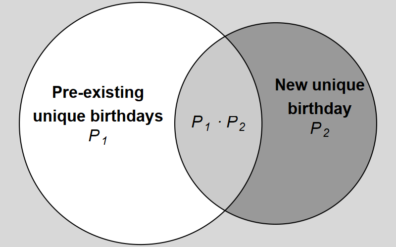
Figure 2: Venn diagram with the events of pre-existing students having unique birthdays (white area, probability P₁) and the incoming student also having a unique birthday (dark grey area, probability P₂). Their overlap is both occurring at the same time, with probability P_(1 AND 2) = P₁ · P₂.

The available birthdays for this added student are 365‑2 out of 365, because it must be different from the 2 existing ones.

So the probability no common birthday at all is: $$\displaylines{P_{no~common~birthday,3} = P_{no~common~birthday,2} \cdot \frac{365-2}{365} \approx \\\ 0.9973 \cdot 0.9945 = 0.9918}$$

Again, we can crosscheck with the precise P_{common birthday,3} we calculated in part 1 (0.0082). $$P_{common~birthday,3} = 1 - P_{no~common~birthday,3} \approx 1 - 0.9918 = 0.0082$$

It also matches, which means we’re on the right track.

Any number of students #

At this point, it’s important to spot the pattern. P_{no common birthday,n} is based on P_{no common birthday,n‑1}. For example: $$P_{no~common~birthday,\color{white}\colorbox{green}{3}} = P_{no~common~birthday,\color{white}\colorbox{purple}{2}} \cdot \frac{365 - \color{white}\colorbox{purple}{2}}{365}$$

This has no reason to stop for any n: $$\bbox[5px, border: 3px solid currentColor]{P_{no~common~birthday,\color{white}\colorbox{green}{n}} = P_{no~common~birthday,\color{white}\colorbox{purple}{n – 1}} \cdot \frac{365 - \color{white}\colorbox{purple}{(n – 1)}}{365}}$$

It’s easier to understand this formula exactly as we built it: by adding students one by one.

Figure 3: Probability of no common birthday in a classroom. Top right pie chart: amount of days in the year that are ‘available’ or ‘taken’ by existing students. Illustration inspired by Wrath of Math’s YouTube video.

Two things come out of this:

1. It vaguely makes sense why P_{common birthday} quickly blows up: the probability of its opposite event quickly shrinks.

   P_{no common birthday} starts from 1 (or 100%), but is multiplied with a smaller and smaller fraction with each added student, speeding towards 0.

2. We just stumbled upon the concept of mathematical recursionNot to be confused with computational recursion, which will not be used in this post.: defining something in terms of a simpler version of itself.

   • The result for any number n is based on the result for the previous number (n‑1).
   • This goes all the way down to the base case of n=1: P_{no common birthday,1} = 1.

Programming: step-by-step calculation of P_{no common birthday} #

Now that we have a recursive formula for P_{no common birthday}, we need to encode it for the computer to calculate and give it back to us nicely organized.

For each n, P_{no common birthday} is essentially all the probabilities P_{new unique birthday} up to that n, multiplied together. In other words:

P_{no common birthday} is the cumulative product of P_{new unique birthday}.

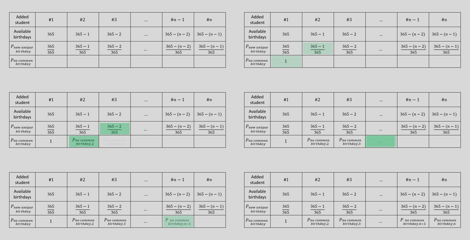
Figure 4: Approach to calculating P_{no common birthday} as the cumulative product of P_{new unique birthday} (merging green boxes: multiplication).

Let’s initiate a data structure similar to figure 4. The code below creates a data table to calculate the probability for up to 50 students.

library(data.table)

# Initiate a data table with one column for the number of students (n)
common.birthday.prob.data <- data.table(n=1:50)

# Calculate the pool of available birthdays for the latest added student
common.birthday.prob.data[,available.birthdays := 365-(n-1)]

# Calculate the probability that the latest added student's birthday is unique
common.birthday.prob.data[,P.new.unique := available.birthdays/365]

# Display the data table
common.birthday.prob.data

##      n available.birthdays P.new.unique
##  1:  1                 365    1.0000000
##  2:  2                 364    0.9972603
##  3:  3                 363    0.9945205
##  4:  4                 362    0.9917808
##  5:  5                 361    0.9890411
## ---                                    
## 46: 46                 320    0.8767123
## 47: 47                 319    0.8739726
## 48: 48                 318    0.8712329
## 49: 49                 317    0.8684932
## 50: 50                 316    0.8657534

The resulting data table is very similar to the one in figure 4, except it is vertical instead of horizontal.

The code below calculates P_{no common birthday} as the cumulative product of P_{new unique birthday}.

# Calculate the probability of no common birthday
common.birthday.prob.data[,P.no.common.birthday := cumprod(P.new.unique)]

common.birthday.prob.data

##      n available.birthdays P.new.unique P.no.common.birthday
##  1:  1                 365    1.0000000           1.00000000
##  2:  2                 364    0.9972603           0.99726027
##  3:  3                 363    0.9945205           0.99179583
##  4:  4                 362    0.9917808           0.98364409
##  5:  5                 361    0.9890411           0.97286443
## ---                                                         
## 46: 46                 320    0.8767123           0.05174716
## 47: 47                 319    0.8739726           0.04522560
## 48: 48                 318    0.8712329           0.03940203
## 49: 49                 317    0.8684932           0.03422039
## 50: 50                 316    0.8657534           0.02962642

Code explanation

We create a new column P.no.common.birthday and assign it the resulting P_{no common birthday}.

This new column is calculated with the cumprod function on column P.new.unique.

cumprod calculates the cumulative product of a vector:

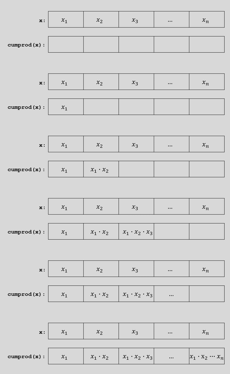
Figure 5: The cumprod function calculates the cumulative product of a vector x with elements x₁, x₂, …, x_n (merging green boxes: multiplication).

The final step is to simply calculate P_{common birthday} = 1 - P_{no common birthday} for each classroom size:

# Calculate the probability of at least one common birthday
common.birthday.prob.data[,P.common.birthday := 1 - P.no.common.birthday]

common.birthday.prob.data

##      n available.birthdays P.new.unique P.no.common.birthday P.common.birthday
##  1:  1                 365    1.0000000           1.00000000       0.000000000
##  2:  2                 364    0.9972603           0.99726027       0.002739726
##  3:  3                 363    0.9945205           0.99179583       0.008204166
##  4:  4                 362    0.9917808           0.98364409       0.016355912
##  5:  5                 361    0.9890411           0.97286443       0.027135574
## ---                                                                           
## 46: 46                 320    0.8767123           0.05174716       0.948252843
## 47: 47                 319    0.8739726           0.04522560       0.954774403
## 48: 48                 318    0.8712329           0.03940203       0.960597973
## 49: 49                 317    0.8684932           0.03422039       0.965779609
## 50: 50                 316    0.8657534           0.02962642       0.970373580

We made it. The column P.common.birthday is the calculated P_{common birthday} that we initially set out to find.

Results: Probability vs sampling frequency #

We can now see how closely we approximated the true P_{common birthday} in part 2. The plot below compares the precise probabilities we just found with the sampling frequencies from part 2:

So the approximate solutions from part 2 are extremely close to the real probabilities. It seems Monte Carlo sampling was a good enough method to reproduce the pattern.

The problem solving triangle #

With a series of three full blog posts, I’ve given an unreasonable amount of thought to this brain teaser. The overarching point I want to make is:

There are different ways to approach the same problem.

And not just vaguely different. The different approaches in this series follow a specific framework.

“Good, fast, cheap. Choose two.” concisely expresses the triple constraint or project management triangle: a model of common constraints in project management: scope, time, and cost.

Looking back on this series, I see a slight variation of this in problem solving. The spectrum of different approaches is roughly shaped by constraints on three factors:

• scope, meaning what we actually get
• time and effort spent
• available resources

The figure below shows how these factors played into each of the three parts in this series. Toggle between parts 1, 2, and 3.

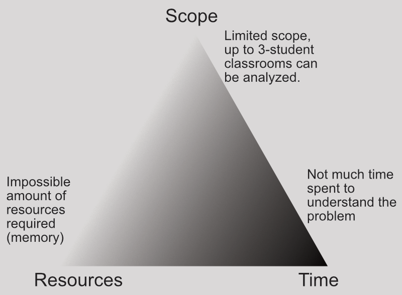
Figure 7: Severity of constraints of our three different approaches on the birthday problem. Light color: limited or high-demand factor; dark color: abundant or low-demand factor.

In this case, we can choose approach depending on our needs and resources:

• Counting: we’re satisfied with an extremely narrow scope or have much, much more computational resources.

• Monte Carlo sampling: we care about being more or less correct and can’t -or don’t care to- approach the problem analytically. Monte Carlo sampling is commonly used for difficult or impossible problems to solve analytically.

• Analytical solution: we want precision and have enough understanding for an analytical approach.

Sometimes perfect is the enemy of good, and cutting corners is necessary to get to a solution. Other times we need the best or most precise solution, and can afford the cost and effort it takes to get there.

No right or wrong. Just scope, time, and resources.

## R version 4.6.1 (2026-06-24 ucrt)
## Platform: x86_64-w64-mingw32/x64
## Running under: Windows 11 x64 (build 26200)
## 
## Matrix products: default
##   LAPACK version 3.12.1
## 
## locale:
## [1] LC_COLLATE=English_United States.utf8 
## [2] LC_CTYPE=English_United States.utf8   
## [3] LC_MONETARY=English_United States.utf8
## [4] LC_NUMERIC=C                          
## [5] LC_TIME=English_United States.utf8    
## 
## time zone: Europe/Stockholm
## tzcode source: internal
## 
## attached base packages:
## [1] stats     graphics  grDevices utils     datasets  methods   base     
## 
## other attached packages:
## [1] plotly_4.12.1       ggthemes_6.0.0      ggplot2_4.0.3      
## [4] data.table_1.18.6.1 blogdown_1.24.1    
## 
## loaded via a namespace (and not attached):
##  [1] gtable_0.3.6       jsonlite_2.0.0     dplyr_1.2.1        compiler_4.6.1    
##  [5] tidyselect_1.2.1   stringr_1.6.0      tidyr_1.3.2        jquerylib_0.1.4   
##  [9] scales_1.4.0       yaml_2.3.12        fastmap_1.2.0      R6_2.6.1          
## [13] labeling_0.4.3     generics_0.1.4     knitr_1.52         htmlwidgets_1.6.4 
## [17] tibble_3.3.1       bookdown_0.48      bslib_0.12.0       pillar_1.11.1     
## [21] RColorBrewer_1.1-3 rlang_1.3.0        cachem_1.1.0       stringi_1.8.9     
## [25] xfun_0.61          sass_0.4.10        S7_0.2.2           otel_0.2.0        
## [29] viridisLite_0.4.3  cli_3.6.6          withr_3.0.3        magrittr_2.0.5    
## [33] crosstalk_1.2.2    digest_0.6.39      grid_4.6.1         rstudioapi_0.19.0 
## [37] lifecycle_1.0.5    vctrs_0.7.3        evaluate_1.0.5     glue_1.8.1        
## [41] farver_2.1.2       httr_1.4.9         rmarkdown_2.32     purrr_1.2.2       
## [45] tools_4.6.1        pkgconfig_2.0.3    htmltools_0.5.9